Don’t judge a book by its cover. -Someone
Did you buy your loved ones presents for this year’s upcoming holidays season yet? Do you have younger cousins, nieces, nephews or children of your own? Are you planning on surprising the younger ones with a book or two? Imagine you are at a bookstore looking for the right gift, trying to decide between two books you saw in the children’s section. Let’s say these are the two books (taken from Amazon’s Children’s Books category):
| Those Darn Squirrels Fly South | Bonyo Bonyo |
|---|---|
 |
 |
Your phone is dead, and the employees of the bookstore are nowhere to be found. Without access to any other information, could you still choose which one to buy just by looking at their covers?
You probably had an intuitive answer to that question, but do you really know why you made that decision? This is what we want to investigate here, using the power of data! Based on their cover aesthetics, could we predict a book’s Amazon sales rank and review score? After all, these two metrics are good indicators of the popularity of the books; maybe your presents won’t be returned this year!
Put on your knitted reindeer jumper, buckle up, and get ready as we take you through our data story which will uncover the scientific answer to the question raised above. This year, we will make sure you are on the same page as the younger ones!
Also, check out the code for our detailed analysis as well as this website’s source code!
Table of Contents
The Data
What do we need to do Data Science? Data, of course!
Data Collection
We have scraped the cover images of, and basic information on, around 13000 books listed on Amazon. The book information has the following format:
| ID | Review Score | Sales Rank | Number of Reviews | Title | Author | Date |
|---|---|---|---|---|---|---|
| ID | Review Score | Sales Rank | Number of Reviews | Title | Author | Date |
Note about the Sales Rank to avoid future confusion: This number represents the book’s placement in the sales rankings of Amazon books, e.g. the number one best seller book would have a Sales Rank of 1. This means that a book with a lower sales rank has been bought more than a book with a higher sales rank.
One thing we had to keep in mind while collecting the data was the book categories. Different types of covers may work better for different categories of books (e.g. dark covers might be good for horror books but not so much for children’s books), and we may see effects in specific categories that are not observable when looking at all of them (and vice versa), i.e. the so-called Simpson’s paradox!

In order to avoid encountering the Simpson’s paradox, we only focused on books from the same category so that our samples come from the same distribution (more or less). We do not want to compare apples to oranges, and this specification allows us to account for the changes in sales and reviews within categories. We intuitively believe children’s books will be the genre that is most dependent on the visual features of their covers, and therefore our analysis will be done based only on these.
Feature Extraction
So, in order to judge a book based on its cover, we will need data that quantifies the cover characteristics! From each image, we extracted the semantically meaningful visual features as shown in the tree plot below.
Before seeing what the features look like for our two book cover examples, let’s quickly break down what each of the features represents:
Brightness: Brightness measure between 0 and 1, where 0 corresponds to a completely black image and 1 corresponds to a completely white image.Colorfulness: Measure of colorfulness adapted from here!Entropy: Measure of entropy of a book cover, which is somewhat an indication of the level of randomness.UniqueColors: The number of unique colors present in a book cover. Each RGB representation accounts for a unique color.Keypoints: Measuring the normalized complexity of the cover by counting edges and corners of the imageColor1R: Amount of red in RGB representation of the most dominant color.Color1G: Amount of green in RGB representation of the most dominant color.Color1B: Amount of blue in RGB representation of the most dominant color.Color2R: Amount of red in RGB representation of the second-most dominant color.Color2G: Amount of green in RGB representation of the second-most dominant color.Color2B: Amount of blue in RGB representation of the second-most dominant color.
Now, let’s investigate the values for our two book cover examples:
| Title | Those Darn Squirrels Fly South | Bonyo Bonyo |
|---|---|---|
| Cover | |
|
| Brightness | 0.83 | 0.52 |
| Colorfulness | 59.8 | 60.3 |
| Entropy | 6.8 | 5.8 |
| UniqueColors | 87982 | 34160 |
| Keypoints | 0.04 | 0.01 |
| Most Dominant Color |  |
 |
| Color1R | 232 | 229 |
| Color1G | 246 | 198 |
| Color1B | 241 | 146 |
| Second Dominant Color |  |
 |
| Color2R | 208 | 237 |
| Color2G | 223 | 212 |
| Color2B | 132 | 175 |
According to the feature UniqueColors, Those Darn Squirrels Fly Down South has more than twice as many different colors as Bonyo Bonyo. The sharp mind probably already noted this the first time when the two covers were presented in the previous section! Also, the colors extracted as the most and the second-dominant ones seem to fit!
Before going directly to the interesting results, let’s first get a closer look at the data.
Exploration
As the first exploratory plot we will examine the distribution of our initial response variable, Sales Rank, and also of the other possible response variable, Review Score.
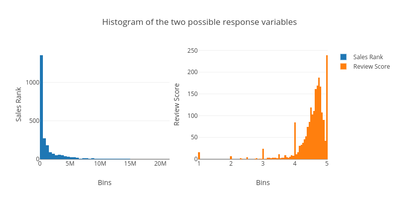
As seen in the above plot, our response variables follow similar patterns to a power law distribution. Just as the literature says, plotting the distribution on a log-log scale the plot distribution becomes almost linear.
In the plot below we examine the correlation between the response variable, Sales Rank and the continuous variable, Review Score.
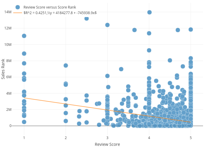
From this plot you can see each book with the Title and the corresponding Review Score and Score Rank when hovering over the datapoints. We can also see a correlation that we would expect to see, which is a positive relationship between sales and review scores. Of course there are popular books that are not well-liked and there are books with excellent reviews that aren’t popular at all, but the general trend seems to show books with better reviews get more sales.
As seen in the above scatterplot, Review Score is not a categorical variable, but it does to an extent act like one. As seen from the above plot there are very few reviews between the integers in the 1-5 scale. This is because Amazon only allows users to give an integer score, so books with only one review or a few reviews with the same score end up on integer average review scores.
Furthermore, since we wish to explore the ability of predicting the Sales Rank or the Review Score based on visual features, a few of the features, Entropy, Brightness, and Keypoints, are visualised against the two proposed response variables.
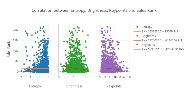
From this we actually see that some of these visual features have some correlation with the Sales Rank. More specifically we see for Entropy that higher values of entropy score tends to give higher sales rank (so worse sales). For Brightness it seems brighter covers lead to more sales (lower sales rank). Lastly, for keypoints, which is another way of calculating a measure of complexity, the more complex the lower the sales rank (more sales). An interpretation of these plots would be that brighter covers catch the attention of the potential buyer and increase the sales, and adding complexity (keypoints) might also help if it is not just making the cover random (entropy).
Let’s examine the same for Review Score:
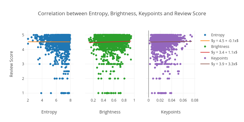
In the figure above, we see a very different pattern for the visual features and the response variable. Again, the plot is affected by Review Score acting like a categorical one for some books.
Based on the plots above, it seems like the visual features alone might be better at predicting the Sales Rank than the Review Score since the features seem to be more correlated to the sales. This also intuitively makes sense: to write a review, buyers must first read the book so their reviews will presumably be more dependent on the content that they went through rather than the cover. Whereas while buying a book, one has access to less information that can be used to decide whether to make a purchase or not, and we believe the cover is among the most important of those pieces of information.
Based on the above exporatory plots we have chosen to focus on the influence of the visual features on the Sales Rank.
Time to judge
To unlock the link between the visual covers and the unknown Sales Rank we will build an ensemble decision tree model: The Random Forest.
The Random Forest is an ensemble of several decision trees. The randomness occurs in the random subsampling of data called bagging. In simple words, the Random Forest will build multiple desicison trees, average the result from all of them in order to reach a more stable and reliable result.
Our aim with this analysis is more than just predicting the Sales Rank with a certain accuracy: the aim is also to understand how the model actually takes in the visual features and how it goes from these inputs to the output. In order to analyze and visualise this, we have used state-of-the-art research, namely the SHapley Additive exPlanations (SHAP) approach.
Below is a bar chart, based on the SHAP value, that shows which visual features have the greatest importance when predicting the Sales Rank. We see that Brightness has almost twice as much influence on the output as the number of unique colors, Unique Colors.

We can visualise the visual feature importance with the plot below. Here we get more insights into which direction the visual features are affecting the prediction of the Sales Rank. The red color represents high values, and the blue color low values. The impact can be seen from the y-axis.
As an example we can focus on again the top 3 features, Brightness,UniqueColors, and, Entropy.

BrightnessSince the output of the model is a rank, the optimal is as low a value as possible. From the above plot we see that the higher values of brightness will result in a lower value of the sales rank.UniqueColorsWe see that the more unique colors the cover has, the lower than rank, and thereby the better the score.EntropyIn contrast to the brightness and the unique colors, higher values of entropy will increase the rank of the sale, and therefore lower values of Entropy is preferable.
So, with this introduction to the model and the results, it is now time to go back to our initial example: which of the initial proposed covers would have a higher Sales Rank?
Let’s refresh our memory with the two covers:
| Those Darn Squirrels Fly South | Bonyo Bonyo |
|---|---|
|
|
Looking at the two bookcovers above it seems like “Those Darn Squirrels Fly Down South” has a significantly brighter book cover, together with more unique colors, and the entropy (randomness) seems to be higher as well.
Further up in this datastory all the visual feature values can be found for these two book covers.
For the sake of simplicity we will focus on the top three features in the light of importance for the Sales Rank.
| Title | Those darn squirrels fly south | Bonyo Bonyo |
|---|---|---|
| Brightness | 0.83 | 0.52 |
| UniqueColors | 87982 | 34160 |
| Entropy | 6.8 | 5.8 |
Just as it seemed like by looking at the covers, it is seen how “Those Darn Squirrels Fly Down South” has a higher value than “Bonyo Bonyo” for the brightness feature. Subsequently, it is seen how the number of unique values are also higher, as well as the Entropy.
So based on our model, “Those Darn Squirrels Fly Down South” should be having a higher Sales Rank compared to “Bonyo Bonyo”. Looking into the ranking for the two books give the following result:
| Title | Those darn squirrels fly south | Bonyo Bonyo |
|---|---|---|
| Sales Rank | 10244 | 1786788 |
Wow… What a relief and what a coincidence! Just almost a factor 200 better ranking than “Bonyo Bonyo”. This example is surely not cherry picked… So, is the model just perfect, or?
Our Model Is Flawed
As you probably already have guessed, our model is not perfect. In the following, we will showcase an example where the model clearly does not work. Also, we discuss general drawbacks of the model.
Tricked by Harry Potter
Since this model only takes in the visual covers, it of course has flaws when it comes to predicting the rank of the sales. Let us take a well-known book as example. We all know the great tales of Harry Potter. One of the books we have in our data set is “Harry Potter and the Sorcerer’s Stone”, which has the following book cover.

Let’s look closer into the features of this book cover.
| Title | Harry Potter and the Sorcerer’s Stone |
|---|---|
| Brightness | 0.48 |
| UniqueColors | 113980 |
| Entropy | 7.7 |
From these features we see that we have lower brightness, and higher entropy than the values of the two other book covers shown in the previous section. On the other hand, the count of unique colors are higher.
And what would we think about the Sales Rank based on these cover features? Two of the features are significantly worse than the ones before, whereas one is better. Maybe it would be in between the ranks of 10.000 and 180.000? Let’s examine…
| Title | Harry Potter and the Sorcerer’s Stone |
|---|---|
| Sales Rank | 188 |
With a sales ranking of only 188 it is clear that our model has some flaws in the way that I does not take any other information about the books into account.
Some More Drawbacks
As we saw in the previous sections, our model and potentially the extracted features clearly do not represent popular books well. One could argue that the more popular a book is, the less the aesthetics of its book cover matter. This observations is potentially a part of a broader problem already addressed earlier – i.e. the Simpson’s paradox!
In order to account for the changes in sales and review within the children’s books category, the books are required to be drawn from roughly the same distributions. As we saw with the Harry Potter example, very popular books are likely to distort the underlying distribution of the books.
In addition, the majority of the books in the children’s books category are likely not appropriate for the same age group, and this could also distort the underlying distribution. If this information was available about each book and was used as a feature in our model, the model performance could potentially be further enhanced.
One other drawback we could not account for is the change of book covers over time. This is of course a limitation to our model, as it relies on the cover found on the book’s Amazon listing at one time.
Other improve points include dividing the books into even more smaller subcategories, and either train a model on each of these categories or incorporate the subcategories as features in a single model.
Conclusion
In this project we have seen that we can extract important visual information about book covers even though they only to a certain degree could work as predictors of the Sales Rank. Specifically, we saw that popularity of books would be a drawback of the model.
In general, good practices among book covers were found to be bright book covers, a high amount of unique colors, together with a low amount of randomness. Of the less important features we saw that more complexity (but not random) would lead to a marginally lower ranking, and the same goes for the red RGB value of the most dominant color in the cover.